The Goldilocks Seasonal Soup (GSS) Company is a food truck that serves soups during lunch and dinner. They try to make their soups at just the right temperature, hence the truck's name. They also try to accommodate the right soups for the right seasons.

GSS is a fictitious company. However, the research about the temperature of soups is real and included here.
Scenario
GSS has discovered that the most popular soups sell quickly, and these are always the hottest.
Due to quick turnover, the truck makes these soups most often. People often burn their mouths when choosing popular soups because they are always hot.

The next popular soups sell well but sit for longer periods than the most popular soups. Ironically, these soups tend to be close to the perfect temperature. They aren’t the most popular, but they are good-selling soups.
The last category of soups is the ones that sit around too long. These are not the most popular with patrons. Since GSS has a limited number of stoves, they cannot keep all soups as warm as possible. They often set aside the least popular soups to make room for the more popular ones.
On occasion, customers will order a least-popular soup. By the time this happens, the soup is cooler than it should be.
The owners of GSS have hired a data analyst (you) to help them categorize their soups by temperature. The management did initial research and found the temperatures of soup is defined in these ranges:
Soups with temperatures:
Under 130 should be labeled as too cold
Between 130 (inclusive) and 170 (exclusive) – Just right
Over 170 should be labeled as too hot
Goals of this tutorial
My goal of this tutorial is to help you learn a few intermediate SQL concepts without getting too detailed in how they work. Just grasp the few concepts before moving onto the next. Window functions have many components to them, but by keeping the concept simple, you’ll grasp the concept quickly.
Don't know SQL? No worries. Learn about a fantastic resource that teaches you data science techniques, including SQL. You are in good hands with your training when you join!
----> Get started now!
Another goal is to choose an environment that is easy to set up or can be run using an online SQL engine. SQLite is the perfect choice for this goal. You can either install a SQLite version (I like DB Browser for SQLite or use the online SQL engine:
In either case, I have included the Soup database on GitHub. Both DB Browser and SQLite Online can access this database. It’s called GoldilocksSeasonalSoups.db.
Whether you're using DB Browser for SQLite or SQLiteonline, simply open the database and you'll have access to the table.
NOTE: the scenario in this tutorial does not consider the pandemic, which would drastically alter the analysis. It would overcomplicate the scenario. The point of the tutorial is to show how certain SQL constructs can be used. When working for actual clients, you would need to take all factors into consideration.
The ranges used for the soup temperatures are based on actual research. However, much of the analysis used is based on random data generated that may not be or may not be applicable to a soup truck business. Please consider this carefully when using this tutorial!
SQL Concepts Used
We’ll discuss the use of window functions using the AVG() aggregation. The window function is helpful as it can aggregate without rolling up by the columns in the select list. This means we can get the temperature amount and the average all in one shot and then see where the temperature fits within the average.
Window Functions with AVG()
SQL has several options when using window functions. The basic concept behind a window function is that it allows the developer to carve out a frame or a window from the result set based on the function's conditions.
Why is this useful? When you submit a query to a SQL engine, you are given the result set in its entirety, based on the conditions (WHERE, etc.) of the query submitted. You do not have access to the row-by-row information. By the time you receive the results, all the row-by-row processing has already been done inside the engine.
Window functions allow you to interrupt that row-by-row processing and apply certain conditions (often aggregations) on the rows before they are returned. The coverage of window functions is beyond the scope of this article. For our purposes, we’ll use only a few of the options.
In many cases, if we want to use aggregations on our data, we apply a GROUP BY clause. However, the GROUP BY rolls up the data based on the columns you specify in the clause. For instance, suppose you wanted to know the average temperatures of soups by season. You could use the following statement:
SELECT season, AVG(temperature) as AvgTemp
FROM GoldilocksSeasonalSoups
GROUP BY season;
Results:
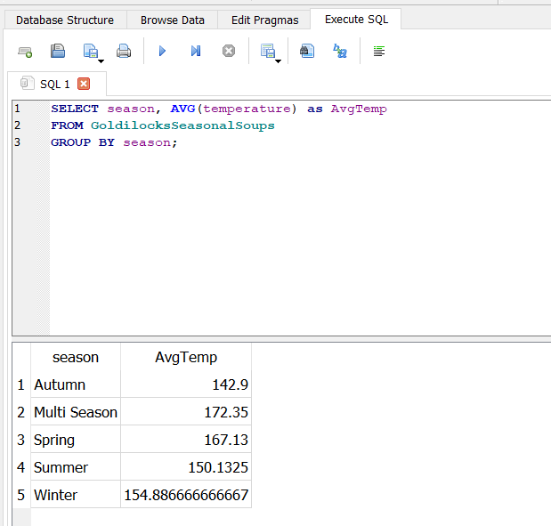
You’ll often use this format when you work in data science or as a data analyst. But what happens if you want to see the components of the aggregation without rolling up the values but also have the aggregated values available? That isn’t something you could do with a GROUP BY statement. For instance, if you remove the GROUP BY:
Select season, AVG(temperature)
FROM GoldilocksSeasonalSoups;
Results:
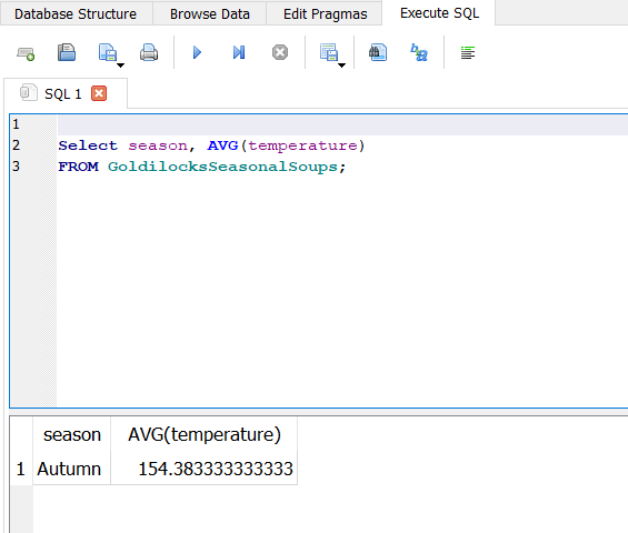
You’ll receive the overall average of the entire database, but it will be associated with the first record, which is incorrect. SQLite allows you to run this aggregation, but it is wrong. Most of the other major SQL engines will flag this statement as an error.
Goldilocks Seasonal Soups owners would like to see how far off from the average each soup temperature is. They can use this information to determine whether to drop a few of the soups that are far away from the average.
They probably won’t drop the hottest temperatures, as these stay hot during the day because of fast turnover. But the management may decide to take action for soups that get taken off the burners to make room for the more popular soups, i.e., the lowest popular soups.
To help GSS with their task, you’ll need a method to get both the soup's temperature and the average of all soups. I’ll discuss later how you can get the average of soups by season using this same concept.
It is entirely possible to accomplish this method using subqueries. However, these subqueries would likely need to be correlated, which means you’ll use information from the outer loop as part of your criteria for your subquery. Doing this is slow because you have to go through each record as specified in the conditions.
Window functions are more efficient and are easy to manage. The following query (with a window function) will return all the rows in the GoldilocksSeasonalSoups table along with the average for the entire table, constrained by conditions of the where clause, etc.
SELECT *,
AVG(temperature) OVER() as AvgTemp
FROM GoldilocksSeasonalSoups;
Results:
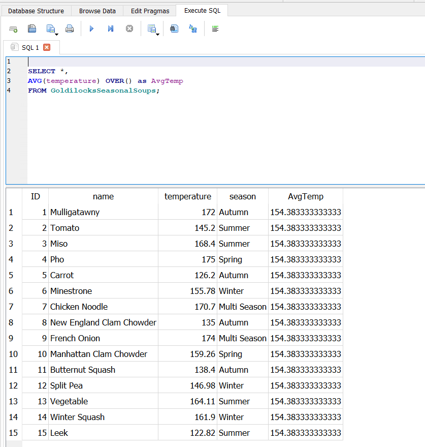
When you run this query, you’ll notice that the AvgTemp column repeats for all the records. However, if you constrained the query for only Autumn records, the average will change:
SELECT *,
AVG(temperature) OVER() as AvgTemp
FROM GoldilocksSeasonalSoups
WHERE season = 'Autumn';
Results:
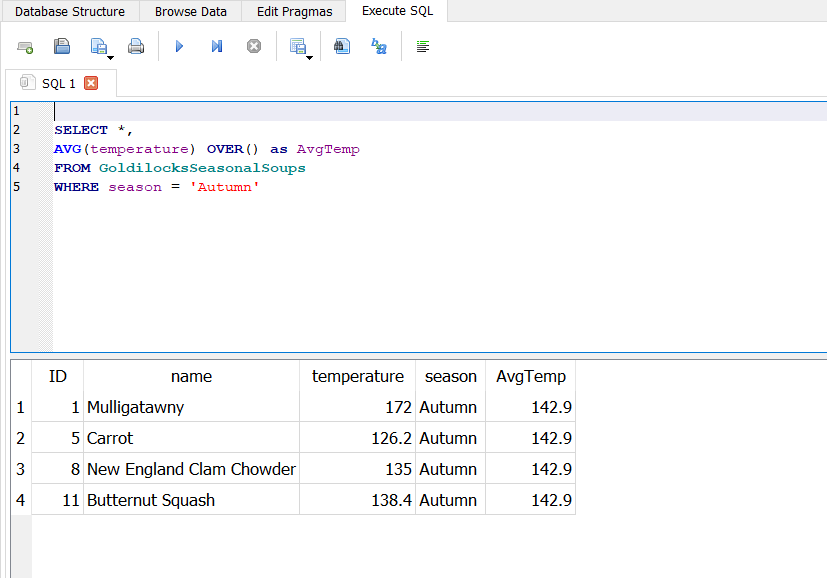
You could try this for all the seasons, and each will change accordingly. For now, though, GSS wants the average of all records.
After you obtain the average of all records, the next step is to subtract it from the soup temperatures. This will result in the difference from the averages. Intuitively, we should be able to subtract the AvgTemp alias from the temperature field and create an alias for that difference. However, this will cause an error:
SELECT *
, AVG(temperature) OVER() as AvgTemp
,temperature - AvgTempSeasonDiff AS DiffFromAverageTemp
FROM GoldilocksSeasonalSoups;
Results:
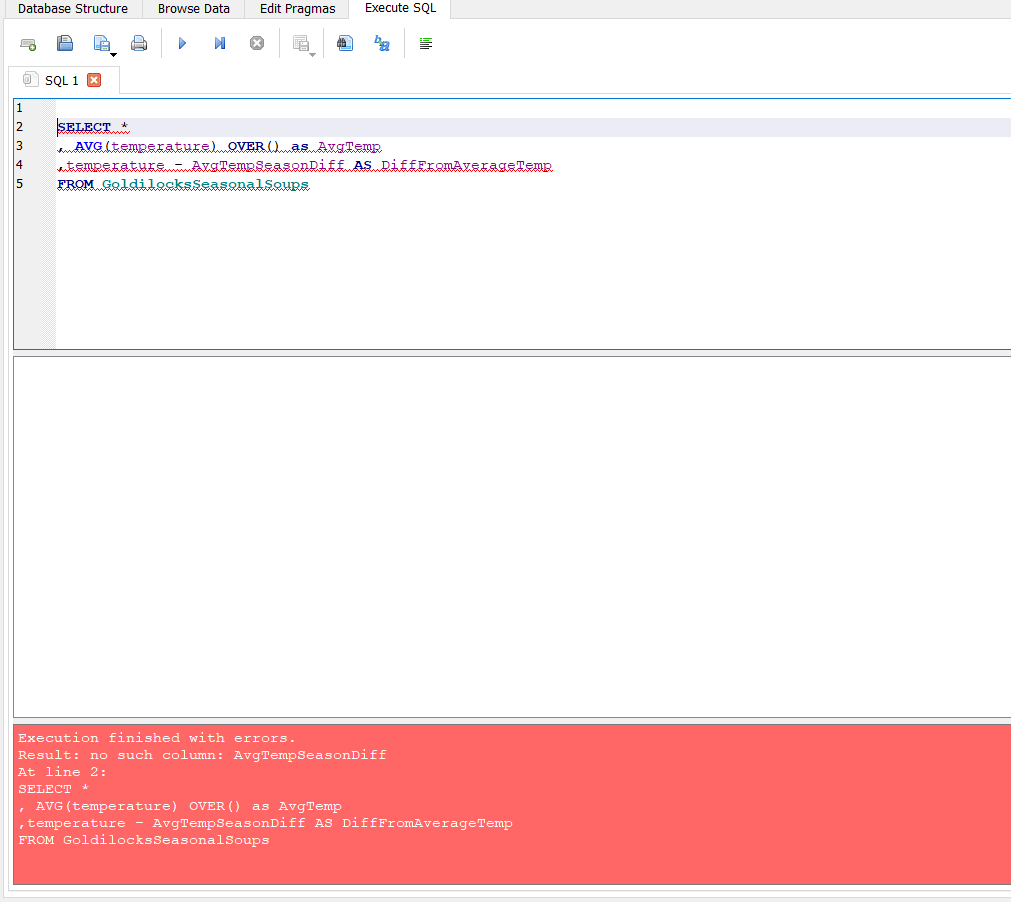
The problem is that aliases don’t yet exist inside the select clause. To get around this problem, we can use the entire window function again in the equation as follows:
SELECT *
, AVG(temperature) OVER() as AvgTemp
,temperature - AVG(temperature) OVER() AS DiffFromAverageTemp
FROM GoldilocksSeasonalSoups;
Results:
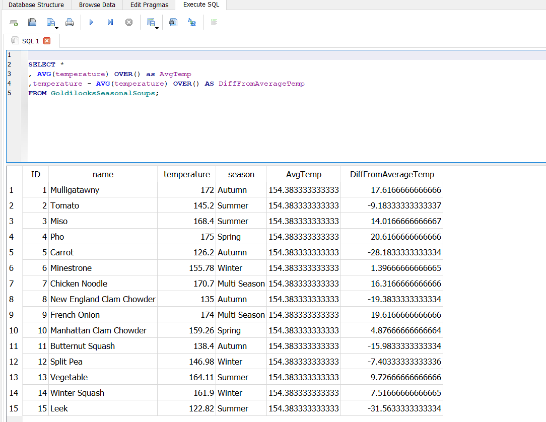
While this works, it can get cumbersome if you need to repeat the window function in several places throughout the select statement. What would be helpful is to find a way to use the aliases created. With Common Table Expressions, that is how we can handle this situation.
Common Table Expressions
A Common Table Expression (CTE) is a bit like a temporary table but is also a bit like a subquery. It is almost like a function call, too.
CTEs allow you to preload queries that you can use further in the main query. You use the CTE to perform specific work units. Since the CTE queries are preloaded, the aliases are available for the main query to use. This is exactly what we need.
To use a CTE, use a WITH {queryname} AS ( -- Query Goes Here -- )
Select * from queryname… etc.
For our soup table, we’ll embed the previous query into a CTE, as follows:
WITH GetAverages AS (
SELECT name, temperature, season,
AVG(temperature) OVER() as AvgTemp
FROM GoldilocksSeasonalSoups
)
SELECT *, temperature - AvgTemp as Diff
FROM GetAverages;
Results:
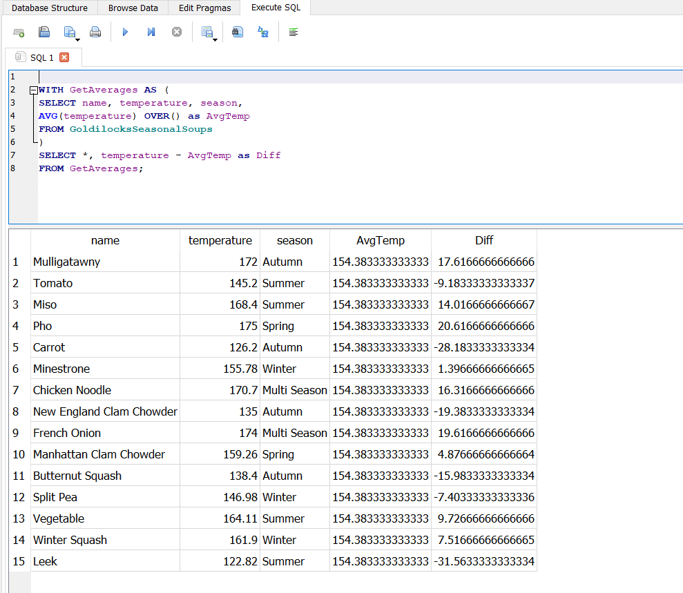
CTEs can be nested. However, you only use one WITH statement (at the start) for the whole series. Multiple CTEs are separated by commas.
Subsequent CTEs are defined by their name and AS ( -- query goes here -- ). The format is as follows:
WITH CTE1 AS ( SELECT * FROM Table1 ),
CTE2 AS ( SELECT * FROM CTE1 )
SELECT * FROM CTE2;
As you can see, you can reference the previous CTEs in subsequent ones. In the above example, CTE1 selects information from Table1 and CTE2 references CTE1 as if it was a table, which for this purpose it is.
CASE Statements
The name of the fictitious soup company is Goldilocks Seasonal Soups. As you may know, Goldilocks was a character who went inside an empty home in the woods. She made herself at home. Three pots of porridge were on the stove, one being too hot, the other being too cold, and the last one being just right.
The management team has asked you to categorize the soups based on temperature into the following buckets:
Soup temperature below 130 – too cold
Soup temperature between 130 (inclusive) and 170 – just right
Soup temperature above 170 – too hot
To create these buckets, you can use a CASE statement in SQL. A CASE statement is like and IF THEN ELSE construct used in other computer languages. It lets you place information into buckets based on the conditions you specify. Here is the syntax:
CASE WHEN {condition1} THEN {action1}
WHEN {condition2} THEN {action2}
…
WHEN {conditionN} THEN {actionN}
ELSE {default condition} END
The ELSE statement is optional, but the END statement is not. For GSS, we can use this CASE statement, testing the temperature based on the criteria above:
SELECT name, season, temperature,
CASE WHEN temperature < 130 THEN 'Too Cold'
WHEN temperature >= 130 AND temperature < 170 THEN 'Just Right'
WHEN temperature >= 170 THEN 'Too Hot'
ELSE 'Something Went Wrong' END AS TemperatureCategory
FROM GoldilocksSeasonalSoups;
Results:
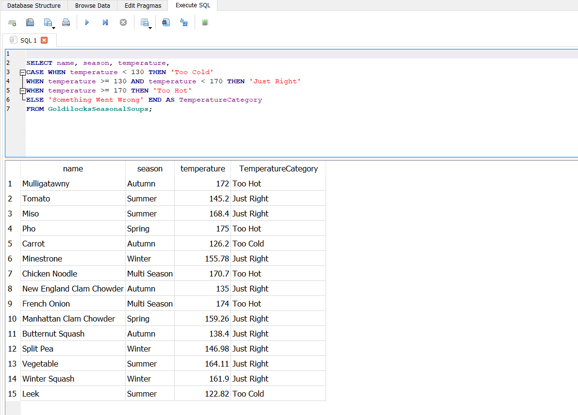
There is nothing to stop you from placing the case statement inside the CTEs you created earlier. The following contains both the window function and the case statement:
WITH GetAverages AS (
SELECT name, temperature, season,
AVG(temperature) OVER() as AvgTemp,
CASE WHEN temperature < 130 THEN 'Too Cold'
WHEN temperature >= 130 AND temperature < 170 THEN 'Just Right'
WHEN Temperature >= 170 THEN 'Too Hot' ELSE 'Unknown' END AS TempCategory
FROM GoldilocksSeasonalSoups
)
SELECT TempCategory, AVG(temperature) AS CategoryTemp
FROM GetAverages
GROUP BY TempCategory
ORDER BY CategoryTemp;
Results:
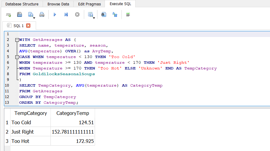
The CASE statement is useful because you can now use the categories in a group by. You will need to place the above code into another CTE if you want to use it in a group by or window function.
Analysis
GSS has asked you to present an analysis of the data. The current analysis calculated the average temperature of all the soups to be 154.38, which was calculated using a window function inside a CTE.
Within the same query, you subtracted the average from each of the temperatures. GSS management wants to determine if they should scrap or replace certain soups that are low temperatures due to removing the soups to make room for more popular ones.

It’s up to them to determine what the line-in-the-sand is for making that determination. It appears that the temperatures of leek and carrot soups are extreme and may be good candidates for replacement. You note this to management.
The management at GSS also requested a categorization of temperatures based on research on the topic. You used a case statement inside a CTE to determine this categorization. This CTE enabled you to group the average temperatures by this newly created category. At this point, you have satisfied the requests of the management of GSS.
However, you feel compelled to provide more to the analysis. The company is located in the northeastern part of the United States. They experience all four seasons of weather. It could be part of the reason for using the word ‘seasonal’ in the company name.
What if you broke down the averages by season? Thinking of your own likes and dislikes with soups, do you eat as much soup in the warmer months as you do in the colder ones? Although this is anecdotal, it’s enough for you to warrant further investigation.
Luckily, window functions make it easy to group with your data components without having to roll up all the data items. That’s what you’ll need for this extra analysis.
Without getting into too much detail about the inner-workings of window functions (beyond the scope), you can include further parameters inside the OVER() function. The parameter we’ll use for this analysis is PARTITION BY. You can also use an ORDER BY with the OVER alongside the PARTITION BY, or in most cases, on its own. But it is a bit more complicated and is not needed for this analysis.
In our case, we’ll PARTITION BY the season, as follows:
WITH GetAverages AS (
SELECT name, temperature, season,
AVG(temperature) OVER(PARTITION BY season) as AvgTemp,
CASE WHEN temperature < 130 THEN 'Too Cold'
WHEN temperature >= 130 AND temperature < 170 THEN 'Just Right'
WHEN Temperature >= 170 THEN 'Too Hot' ELSE 'Unknown' END AS TempCategory
FROM GoldilocksSeasonalSoups
)
SELECT name, season, temperature, AvgTemp
, temperature - AvgTemp AS AvgTempDiff
FROM GetAverages;
(Bold and Red lettering for emphasis)
Results:
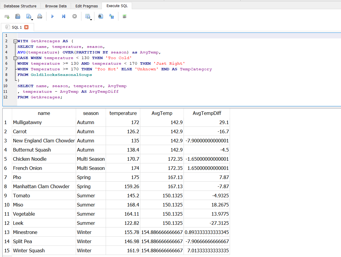
You’ll notice that the lower temperature differences to the average are a bit smaller when seasonality is taken into account. Interestingly, the hotter soup temperatures are a bit more extreme when you factor in the season. This is information that GSS management may find useful.
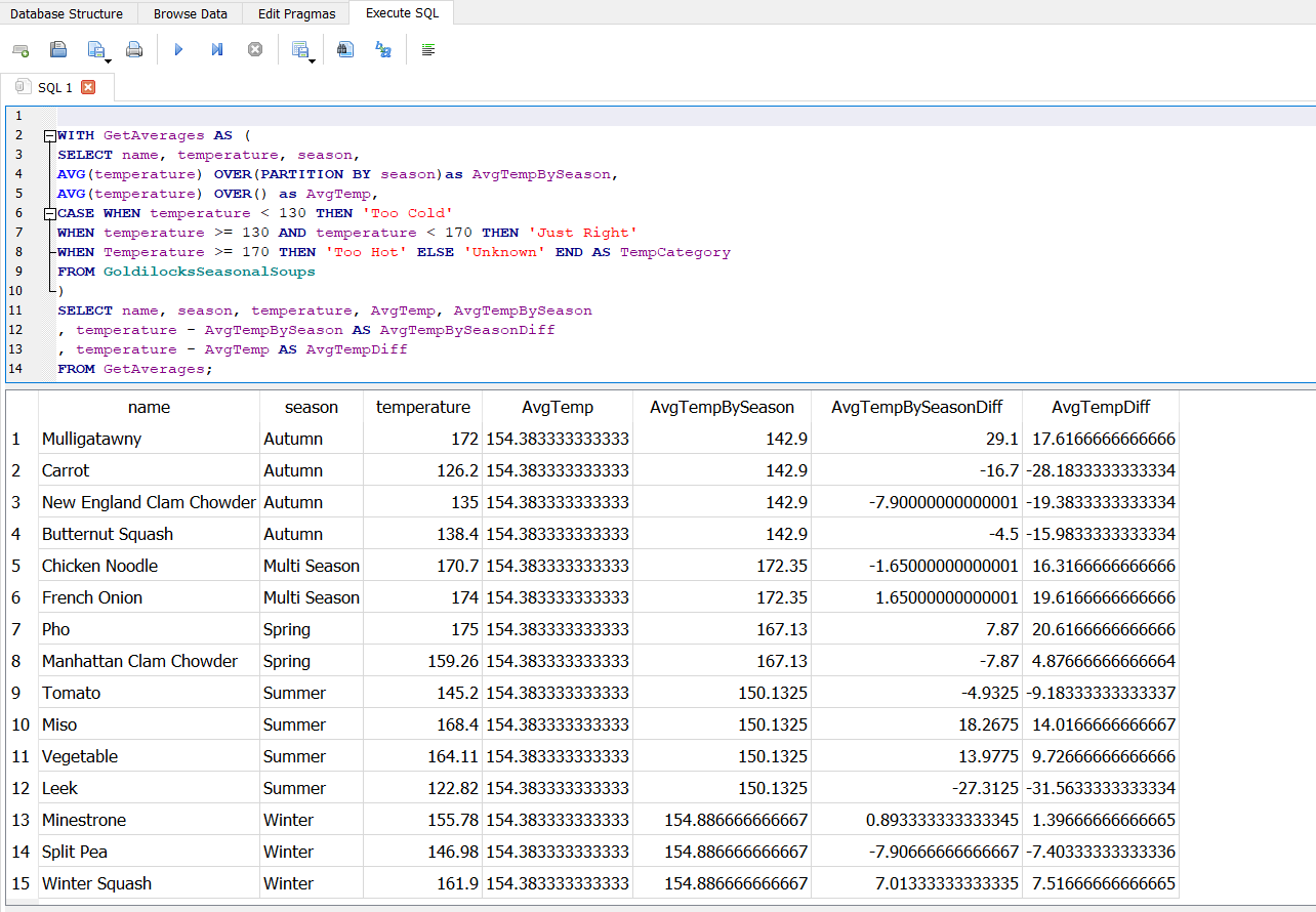
If you wanted to show GSS management the differences in the averages of overall and by season, you could add more window functions within the same CTE. The following calculates the averages by season and the overall average. It also calculates the differences of the temperature field between the two averages:
WITH GetAverages AS (
SELECT name, temperature, season,
AVG(temperature) OVER(PARTITION BY season) as AvgTempBySeason,
AVG(temperature) OVER() as AvgTemp,
CASE WHEN temperature < 130 THEN 'Too Cold'
WHEN temperature >= 130 AND temperature < 170 THEN 'Just Right'
WHEN Temperature >= 170 THEN 'Too Hot' ELSE 'Unknown' END AS TempCategory
FROM GoldilocksSeasonalSoups
)
SELECT name, season, temperature, AvgTemp, AvgTempBySeason
, temperature - AvgTempBySeason AS AvgTempBySeasonDiff
, temperature - AvgTemp AS AvgTempDiff
FROM GetAverages;
Results:
Join a Leader in SQL Training
Learn about this premiere resource for learning data science, including SQL.
Conclusion
Hopefully, this tutorial has helped you recognize (and use) powerful constructs in the SQL language. All the techniques described here should work in all the major SQL engines. You learned how window functions, CTEs, and CASE statements could be used to perform a rather sophisticated analysis.
It wasn’t meant to be extensive coverage on any of these topics. It’s just meant to show you some of the possibilities and pique your interest in learning more.
Resources:
"How to Bucket Data in SQL." Data Science Review, 8 December 2020, https://datasciencereview.com/how-to-bucket-data-in-sql/
Reilly, Lucas. “The Perfect Temperature for Soup, According to Science.” Mental Floss, 6 Jan. 2020, www.mentalfloss.com/article/609356/whats-the-best-temperature-for-soup.

