- You are here:
- Home »
- Business Intelligence »
- Mastering USERELATIONSHIP() in DAX: A Deep, Practical, and Engaging Guide
Mastering USERELATIONSHIP() in DAX: A Deep, Practical, and Engaging Guide
How to unlock alternate relationships and take full control of your data model’s behavior
Power BI’s data model is built on relationships—those invisible highways that let filters flow from one table to another. Most of the time, the model’s active relationship does exactly what you need. But real-world data is messy, multi‑dimensional, and full of competing timelines and lookup paths.
That’s where USERELATIONSHIP() comes into play. It’s the DAX equivalent of saying:
“Hey, Power BI. Use this relationship for this calculation, even if it’s not the active one.”
This tutorial will walk you through not just how USERELATIONSHIP() works, but why it exists, when to use it, and the subtle rules that can trip up even experienced modelers.
RELATED: Want comprehensive training on Power BI? Get started on this beginner-friendly training today.
Disclosure: this affiliate link helps us pay for the cost of the website, but does not add any extra cost to the service.
What USERELATIONSHIP() Actually Does
According to Microsoft’s documentation, USERELATIONSHIP() activates an existing relationship for the duration of a calculation. It doesn’t return a value—it simply modifies filter context.
Syntax
DAX
USERELATIONSHIP(<columnName1>, <columnName2>)
Both arguments must be fully qualified column names that already participate in a relationship.
Why USERELATIONSHIP() Exists
Power BI allows only one active relationship between any two tables.

But many datasets have multiple valid join paths. For example:
- OrderDate vs ShipDate
- InvoiceDate vs DueDate
- EmployeeStartDate vs EmployeeTerminationDate
You can only mark one as active. The others become inactive—but still usable with USERELATIONSHIP().
When You Need USERELATIONSHIP()
USERELATIONSHIP() is only allowed inside functions that accept a filter argument, such as:
- CALCULATE
- CALCULATETABLE
- Time intelligence functions like TOTALYTD, CLOSINGBALANCEMONTH, etc.
This makes sense: USERELATIONSHIP() modifies filter propagation, and filters only exist inside these functions.
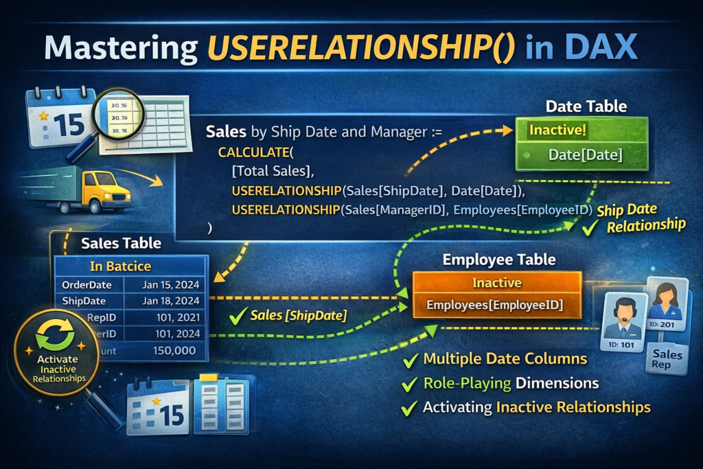
A Classic Example: Switching Date Paths
The official documentation gives a perfect scenario:
Your model has:
- Active relationship:
- InternetSales[OrderDate] → DateTime[Date]
- Inactive relationship:
- InternetSales[ShippingDate] → DateTime[Date]
You want to slice sales by ShippingDate instead of OrderDate.
Solution
DAX
InternetSales by ShippingDate := CALCULATE(
  SUM(InternetSales[SalesAmount]),
  USERELATIONSHIP(InternetSales[ShippingDate], DateTime[Date]))
This temporarily activates the ShippingDate relationship for this measure only.
How USERELATIONSHIP() Chooses the Relationship
A few important nuances from the documentation:
✔ It uses existing relationships—even if they’re inactive
USERELATIONSHIP() doesn’t care whether the relationship is active or not. If it exists, it can be activated.
✔ It identifies relationships by their ending point columns
This means:
- The order of the columns doesn’t matter
- DAX will swap them if needed
- Both columns must belong to the same relationship
✔ If the columns don’t belong to a relationship, DAX throws an error
Multiple Relationships? Use Multiple USERELATIONSHIP() Calls
If your calculation needs to traverse multiple inactive relationships, you must activate each one individually:
DAX
CALCULATE(    [Some Measure],
 USERELATIONSHIP(TableA[Key1], TableB[Key1]),
 USERELATIONSHIP(TableB[Key2], TableC[Key2]))
Each USERELATIONSHIP() activates one relationship path.
Nesting Rules: The Innermost USERELATIONSHIP() Wins
If you nest CALCULATE() calls and each contains a USERELATIONSHIP(), the innermost one takes precedence in case of conflict.
This is subtle but powerful.
One-to-One Relationships: Direction Matters
In 1:1 relationships, USERELATIONSHIP() only activates the relationship in one direction.
If you need bidirectional filtering, you must explicitly activate both directions:
DAX
CALCULATE(    [Measure],
 USERELATIONSHIP(T1[K], T2[K]),
 USERELATIONSHIP(T2[K], T1[K]))
This is one of the most overlooked nuances.
🚫 When USERELATIONSHIP() Cannot Be Used
❌ Row-Level Security (RLS)
If RLS is defined on the table containing the measure, USERELATIONSHIP() will throw an error.
This is because RLS locks down filter propagation rules.
Common Pitfalls and How to Avoid Them
⚠️ Pitfall 1: Forgetting the Relationship Must Already Exist
USERELATIONSHIP() cannot create relationships. It only activates them.
⚠️ Pitfall 2: Using Expressions Instead of Columns
Both arguments must be columns, not expressions or calculated columns.
⚠️ Pitfall 3: Expecting It to Work Outside CALCULATE()
USERELATIONSHIP() is useless unless wrapped in a filter-modifying function.
⚠️ Pitfall 4: Assuming It Overrides All Active Relationships
It only overrides relationships between the two tables involved.
Mental Model: How to Think About USERELATIONSHIP()
You can loosely think of USERELATIONSHIP() as a detour when traveling on a road insofar as it’s not a permanent change.

Admittedly, the analogy weakens as detours are often removed once the road is fixed. For USERELATIONSHIP(), that “detour” will always exist. But the idea is that the functionality does what it needs to do, and then the original relationship is restored immediately after.
USERELATIONSHIP() is like a temporary detour sign:
“For this calculation, use this road instead.”
Practical Patterns You’ll Use Often
📌 Pattern 1: Alternate Date Dimensions
- Order Date
- Ship Date
- Invoice Date
- Due Date
📌 Pattern 2: Multiple Lookup Paths
- CustomerKey vs AlternateCustomerKey
- ProductKey vs ParentProductKey
📌 Pattern 3: Historical Snapshots
- EffectiveDate vs ExpirationDate
USERELATIONSHIP() is essential for any model with multiple valid join paths.
Final Thoughts
USERELATIONSHIP() is one of those DAX functions that separates “report builders” from “data modelers.” It gives you precise control over filter propagation and lets you build measures that reflect the real-world complexity of your data.
Once you internalize how it works, especially the nuances around nesting, directionality, and relationship identification, you unlock a whole new level of modeling power.
About the Author James
James is a data science writer who has several years' experience in writing and technology. He helps others who are trying to break into the technology field like data science. If this is something you've been trying to do, you've come to the right place. You'll find resources to help you accomplish this.
