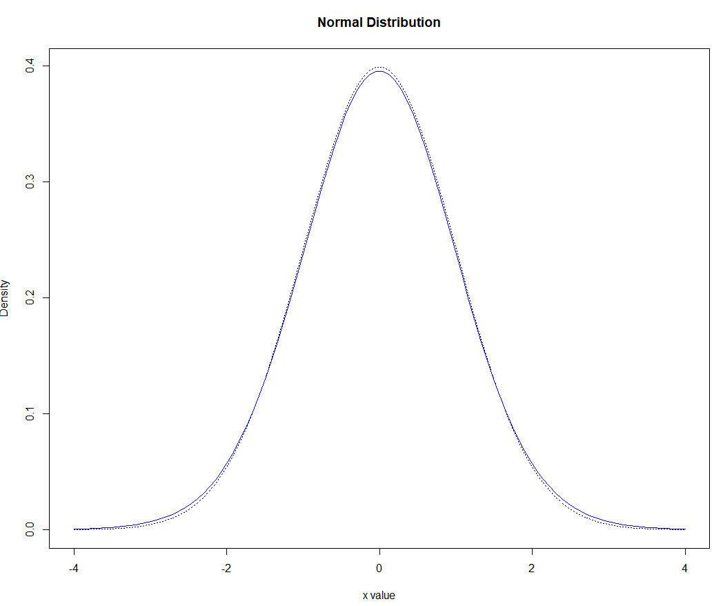
Remember that statistics class that you thought was useless back in college? Bet you didn’t think you’d ever use it once you finished, right? You had to take it as part of the curriculum, but once it was done, you were done with statistics forever, right? It turns out, some of the techniques they taught in that class are quite useful and can be used to generate simulated sales data.

Why Simulate Sales Data?
You may be thinking, why would anyone want to simulate sales data? If you have built up sales data for your business in the past several years, you would use that instead of mock data, and you should.
But what if you were tasked with evaluating a new analytics package and you haven’t accumulated much in the way of data? The more data you have with these tools, the better your evaluation will be for the software. By simulating realistic data, you can put the tool to the test.
NOTE: the link referred to in the video brings you to this article that you are currently reading. Here is the link, anyway, just in case it seems confusing:
https://datasciencereview.com/using-statistics-to-simulate-sales-data/
Another reason to generate sales data is to prove out a concept for your company. You could generate what-if scenarios using data to support your hypothesis. Realistic data will go a long way in that support.
If you are a data consultant, you could generate simulated data to show potential clients how their data could be used for analysis. The more realistic this data, the higher the chances that they will accept your proposal.
I am confident you could find other use cases for simulated sales data. It’s likely you’ll need to generate mock data at some point.
Related: How to Find Your Use Cases
Before we continue, I want to point out the methods used in this article were all written in the R language. As you’ll read later, R handles distributions in a much easier way than Excel does. If you don’t know R, my suggestion would be to check out training on the basics of the language.
You can downloadthe code for this project: Download the Code on My GitHub Page
Can We Talk Normal?
In a previous post, I wrote about how to generate mock sales data. In the post, I described a method that can generate simulated sales data. The method I described worked, but it wasn’t efficient. Statistics gurus would probably look at the method and ask why I didn’t just use normal distributions for my random number generation? They’d be right, too. In many cases, the normal distribution is a much better way to handle this capability.
Why a Normal Distribution Works Better
The technique I described in that last article had you guessing as to the probabilities of each of the components. For instance, to generate the number of products per line item, I set the probabilities at 70% for a one product purchase, 17% for quantity two of a product, 10% for quantity three, and 3% for quantity four. Are these quantities correct? Who knows? Although these probabilities can be adjusted, there is no provision for purchasing quantities greater than four of a product.

With a normal distribution, there is no need to worry about probabilities as they are implied by the mean/standard deviation. For instance, for the product quantities, you can simply use quantity of 1 as the mean. You can experiment with the standard deviation to disperse the numbers generated beyond the mean. The smaller the standard deviation, the more numbers will be generated towards the mean.
An alternative to using the normal distribution for something like product quantity is to use a Poisson distribution. This is usually a better fit for small numbers like quantity purchased (on a daily basis). The random generator is easy enough to swap. Just use rpois instead of rnorm.
Using a normal distribution for your random number generation can help answer the problem of purchasing product quantities larger than 4. But how does it help in generating the most popular products?
To answer this question, start by assigning sequential numbers to your products. This will serve as an index to the products table. You are welcome to assign an alternative field that is not numeric (for instance, SKU numbers). However, it is usually a good idea to index your data using a sequential number. Companies often change how they designate their keys for tables.
When you designate an arbitrary index such as sequence numbers, you can make all the changes you want to other fields that serve as secondary keys. The primary keys won’t change. If you depend on indicators (such as SKUs) as your primary keys, you would need to create a mapping table if changes to the schema were required. Trust me when I tell you this is a maintenance nightmare!

Assigning a numeric sequence to your data also has the advantage that the mean for your normal distribution can represent the numeric sequence of your top-selling product. For instance, suppose your company has five products, Widget-V, Widget-W, Widget-X, Widget-Y, and Widget-Z. Further, suppose Widget-W is the best seller, followed by Widget-Z, then followed by Widget-Y. While you may be tempted to assign the sequence number in order (Widget-V = 1, Widget-W = 2, etc.) you are better off assigning numbers in clusters for the top sellers. Here is what I mean by this:
You have five numeric numbers to assign and they should be sequential. Here is how you may choose to assign the numbers (followed by the reasons why for this schema):
Widget-V = 1
Widget-Z = 2 (second top seller)
Widget-W = 3 (top seller)
Widget-Y = 4 (third top seller)
Widget-X = 5
You would then assign the mean to be the sequence of the top-selling product (in our case Widget-W = 3). When you generate the normal distribution, it will naturally select Widget-W the most number of times (most of the time), due to the nature of normal distributions. The second top products, Widget-Z and Widget-Y, would appear more frequently than Widget-V and Widget X.
The only drawback to this approach is when Widget-Z and Widget-Y have large disparities in the number sold or the price. However, if there are large disparities, you may have to use a different method of generating random numbers than the normal distribution. In most cases, for the purposes of generating mock sales data, the normal distribution should serve you well. Be aware of this bit of a twist, though.
Once you have the mean, experiment with the standard deviation. If you want the numbers to stay close to the mean, run the normal random generator with lower standard deviations. If you want them more spread out, simply increase the number.
Just like the last article on mock number generation, I tried to make this work in Excel. You could use the NORM.INV() function, but you’d have more work to do than running this command one time. In R, you can run the rnorm() function and get it to do much of the work you need.

With the base R functionality, you would have to adjust rnorm() when the items go beyond the bounds of your sequence numbers. For instance, for our product number generation above, the sequence is from 1-5. However, the normal distribution with a larger standard deviation may (and probably will) generate numbers less than one and greater than 5. If you were to simply truncate the numbers, then you won’t have enough numbers for your sales data.
For instance, if you were to generate 1000 products sold to be added into your orders (or sales) table, by truncating the outliers, you’ll have less than 1000 numbers. Your goal of having 1000 numbers to add to your orders table will fall short.
One solution that I tried was to take the total number of outliers and increase the frequency of the mean by that number. Then, when I truncated the lower and upper outliers, the number of records generated matches the number of orders desired.
A better solution is to have a method that bounds the normal random generator. There is an R package that fits the bill. The package is Runuran and the function is urnorm. The first set of parameters are the same. The last two are the lower and upper bounds respectively.
Using this latter solution, to generate 1000 products to be input into the orders table, you could run the following:
Products <- as.integer(urnorm(n=1000, mean = 3, sd = 2.4, lb = 1, ub = 5)
This is all you would need to do to generate 1000 numbers that represent products that can be plugged in directly to your orders table. These products will (for the most part) contain more of the better selling products.
Scenario
You have 234 customers available in your worksheet or database. Your task is to fill 2000 orders with a distribution of the 234 customers. My database just happens to have 234 customers, which is why I used that number. You can adjust to your scenario.
Since you have less customers than the number of orders, you’ll have repeat customers. For many vendors, this is not unusual. For some vendors, like high-ticket items, it would be not as applicable.

For vendors where repeat customers are relevant, you can use a normal distribution. Although customers are considered counts (number of customers within a defined timeframe), there are more than 30 customers, which makes the normal distribution a better choice than the Poisson. The Poisson is meant for counts, but usually for small sample sizes. Feel free to try a Poisson distribution though. The dynamics are similar (rpois(2000, mean)). Since the sample size is larger than 30, we’ll stick with the normal distribution for this example.
Suppose your customer table contains 234 records. These records are sequenced from 1-234. We’ll assume they are consecutive, too, which may or may not be a good assumption. If not, you’ll have to account for gaps as a random distribution could generate customer IDs in your table.
The task is to create enough customer IDs to fill the order table, which for this example is 2000 line items. Since there are only 234 customers, we’ll need to repeat the generation of customers. This coincides with having repeat customers.
To keep this more realistic though, some customers will return many more times than other customers. These can be captured by a normal distribution. As there are 234 customers, we’ll estimate the average at 234/2. This is reasonable for customers who have consecutive numbers from 1 – 234. With this scenario, customer number 117 (234/2) will be the customer who makes the most purchases.

For the purposes of generating mock data, repeat visits always result in a purchase. I realize there is value in knowing which customers visited and didn’t make purchases. That is certainly easier to do with online stores. But it overly complicates the model concerning mock sales or orders. Of course, if the visit to purchase ratio is what you are modeling, you’ll have more work to do to model that. For this model, a visit generates a sale and a sale is one or more products for one or more quantities of the product.
Are repeat visits normally distributed? Probably not. It would largely depend on the type of store. A computer store won’t likely sell multiple computers to a consumer but may sell them to corporations. But even with corporations, the distribution may or may not be normal.
Repeat purchasers on Amazon, on the other hand, may be normally distributed. There are plenty of people who buy items regularly such as pet food and cat litter, ink cartridges, and other items that need replenishing on frequently.
If you are modeling a vendor that has customers with frequent purchases, then you could likely get away with a normal distribution for your customer generation. We’ll assume that to be the case for the purposes of this example. It is after all, meant to show you how to generate random numbers with normal distributions. You can adjust the distributions depending on your needs or circumstances.
If customer 117 ends up with too many repeat visits, that may seem too unrealistic. Try dispersing the data using a higher standard deviation. If you have control over the number of customers, you could also add more customers using a service like Mockaroo.com or something similar. You may not have control over the number of customers, though. A third option is to generate less records for the overall orders, but that too, may not be practical.
We’ll proceed with the assumption that customer repeats are normally distributed, hence our use of the rnorm() function.
Each line item in the order table represents a product purchased, along with the quantity of that product.
As mentioned, the customer ID field in the orders table will be filled in with repeats of customers, since 234 is less than the overall number of orders (2000).
I’ll show the code and then explain each line:

The variable n is the number of customers to generate to add to the orders.
The numCustomers is the number of overall customers with sequence from 1-234. The customerIDMean is the numCustomers / 2.
The customerIDs variable is where we’ll generate the normal distribution. Pass in n, customerIDMean, and for this example, use 35 for the standard deviation. Feel free to adjust this number.
The next two lines handle what happens when the numbers generate dfall outside of the customer ID range. We need 2000 numbers between 1-234 (with repeats). Normal distributions can go past the range, even if the frequency is low. It’s not unusual to see values of 0 or -1 and values that are greater than the maximum number of customers (in this case 234). These two lines will add the frequency of these outliers as the mean and then trim off the outliers. This will have the effect of keeping the number of records generated to n as well as bounding the numbers to the customer IDs (1-234 in our example).
It is possible that not all the values farther away from the mean will be generated. For instance, the customers 1, 2, 4, and 7 (arbitrary) may not exist in one run of code. In another, values over 225 may be sparse as well. There could be instances were both sides of the normal curve are sparse.
This situation is fine as not all customers will purchase. Perhaps they signed up while browsing the website, but decided for one reason or another not to make a purchase. This may seem like a contradiction to an earlier paragraph that stated that a visitor constitutes a sale. But that was only in regards to repeat visitors. It’s valid to have customers in the table but not make any purchases at all.
Why the Distribution May Not Appear as “Normal” as It Should
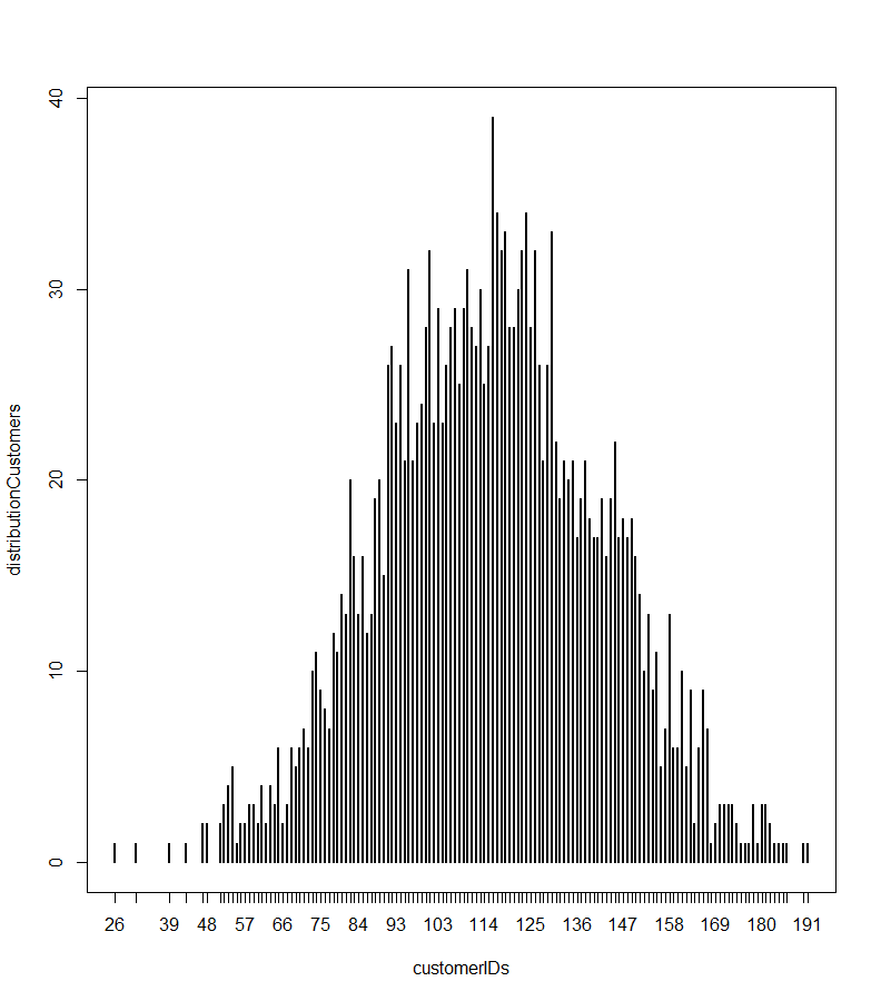
I have included code to plot the distribution. It uses the table() function in R which is a frequency distribution. The chart we generate is normal-ish. But it seems as though there are plenty of values that spike outside of the normal curve. Take a look:

Why Doesn’t This Chart Look More Normal-ish?
There is nothing wrong with the rnorm function. It’s operating as it should. Part of the reason has to do with a statistical concept known as the law of large numbers. Essentially, as the data samples get larger, the mean converges towards the mean of the population.
https://www.investopedia.com/terms/l/lawoflargenumbers.asp
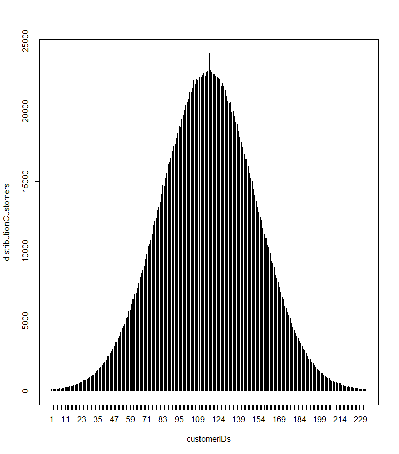
The next image shows the same code but run with n = 2,000,000. As you can see, it looks much closer to what a normal distribution should look like. The big spike in the middle is because of the adjusting of the outliers.
How to Use the Data
Once you generate the random numbers, you’ll need to extract them from R. A fast and easy way to do this is to convert the data to a data frame and write the results into a CSV file. Then, you can load it into Excel, copy the column of values that get loaded, and paste them into your order spreadsheet.
The steps can be combined as follows:
write.csv(as.data.frame(customerIDs), “customers.csv”, row.names = FALSE)
When you create other fields like products and product quantities (either with normal distributions or some other way), you can create a data frame with all the fields and then save the entire data frame to a CSV. This allows you to do all (or at least most) of the work in R.
Suppose you created three variables, productIDs, customerIDs, and productQuantities, set up the data frame as follows:
ordersDF <- data.frame(productIDs, customerIDs, productQuantities)
Then, write the file:
write.csv(ordersDF, “orders.csv”, row.names = FALSE)
Do You Have to Install R?
Most R users have learned about R Studio, as this is one of the best graphical user interfaces (GUI) for R programming. One feature that R Studio offers is a cloud-based interface. It’s actually the same interface as the local desktop version. The good news is that you don’t need to install R on your local drive. You only need an account on the R Studio website, and you’re good to go.
You can install most standard CRAN packages and you can read or write files to your local cloud space. I tried the code published in this article, and it worked fine, including writing out the CSV file.
Conclusion
Using statistics to generate sales data is a great way to make your data more realistic. You need to use the right distributions for the type of data you are generating. As was shown, customer IDs may or may not be a good candidate for normal distributions. But knowing how to use functions like rnorm can be incredibly useful for many scenarios. Due to this, it’s still worth trying out generating customers using a normal distribution.


