Now that the Superbowl is over, we're gearing up for the baseball season. Why not brush up on your favorite players and learn R coding at the same time? In fact, you could be learning R using DPLYR and Baseball stats.

R can be a tricky language to learn. I know because I tried several times before getting the hang of it. The language intriqued me, but it always eluded me when I tried to learn it.
I first learned about it in 2006 when I picked up the book Baseball Hacks by Joseph Adler. It opened my eyes about available baseball data on the internet. But trying to muddle through the R coding was challenging. And I am a programmer by trade!
Then, one day, I simply decided to buckle down and push through my roadblock with the language. I think by the time I was at that point, more decent tutorials were available, making it a bit easier to learn.
Anyone who has read this website knows that now I know love the language.
What I love the most is the subsetting and elementwise processing. You can do so much in a few lines of code.
Aggregation Challenges
After I practiced and got a good handle on the language, the aggregation features left a lot to be desired. Aggregation is the grouping of data that reflects a different (usually higher-level) angle for the data. Summarizing sales regions would be good example for sales-related tables.
When trying to aggregate using the base language in R, it was tedious and slow. Then, I learned about DPLYR. This transformed the way R coders used the language. Aggregation was no longer a chore.
What About Baseball?
One of my reasons for choosing R for this project is a baseball library is available. Can you use this data in Python? Of course. But, to explain how to obtain the library for Python, then the code to load it, is more of an effort. I wanted to hit the ground running without too much background info.
This is all you need to do for R:
install.packages("Lahman")
library(Lahman)
You now have the baseball data downloaded and loaded into your environment. Next, well do the same with DPLYR.
install.packages("dplyr")
library(dplyr)
Yep! You guessed it! You are now ready to start learning R using DPLYR and Baseball stats. Pretty cool, huh?
Using a Baseball Quiz Website
I have to admit. When compiling this tutorial, I was hardpressed to come up with scenarios to use to explain the code. I wanted to use scenarios that you would actually find useful.
One day I found a baseball trivia website and a lightbulb went off in my brain. I started using R to answer the questions. Then, I started incorporating DPLYR to answer the questions that required using aggregation to arrive at the answer.
The great part about this is you can hit up the trivia website whenever you want to practice your R (and by extension DPLYR) coding.
Let's Get Started!
DPLYR Overview (Short!)
I am not going to go into too much detail about DPLYR. It's not difficult to learn. But, describing it has the potential to fill up an entire blog post. Therefore, I will concentrate on quickly describing the features of the package we'll be using to analyze baseball. I will explain as I use the concepts, which will help you learn it even quicker.
I am also going to assume you have basic R knowledge. There are many tutorials available that will show you the basics. Once again, anywhere I believe needs explanation I will do so within the examples. I will provide learning resources at the end of this article for those who need to learn the basics.
DPLYR has six main constructs, with four of them used for this tutorial (*). They are:
- select - select a subset of columns
- mutate - add or change columns based on formula you define
- summarize (*) - aggregate data, can be functions such as sum, mean, etc.
- arrange (*) - another term for sort use desc() for descending order
- filter (*) - add conditions, such as year or games > then a certain number
- group_by (*) - part of the aggregation to determine how to group your data
One other construct you should learn is the pipe operator. The pipe operator (%>%) is defined in the magrittr library, which is included automatically when you load dplyr.
The pipe operator gives you a shorthand notation to pipe results of one command into another. It's often used with dplyr commands to nest together multiple constructs.
For instance, suppose you wanted to find the total homeruns for players in the year 2016:
Batting %>%
filter(yearID == 2016) %>%
group_by(playerID) %>%
summarize(sumhr = sum(HR))
Other DPLYR Concepts...
A few pointers here: in the filter() statement, you'll see double equal sign (==). This is how R does comparisons for equality.
The single equals sign in the sumhr = sum(HR) is an assignment.
It's common for newbies to forget the double equals when making comparisons. The good news is the R interpreter won't let you get away with it and will report an error.
The above code groups by the playerID field. Later, I'll show you how to add the player's full name to the database and then you can group by the name. This isn't always a good idea, though, as it can cause trouble when multiple players share the same name. It will end up summarizing the data for the multiple players together.
When we get to the section where I start grouping by name, I will show you an example to illustrate the problem. There is an easy solution, too. Woohoo!
Don't get too hung up on the command if you aren't familiar with the syntax. When you try a few examples, it will become second nature. Not much will change with the syntax. A few parameter tweaks here and there. But mostly, it's similar from one example to the next. For now, take a leap of faith. Trust me, it really is easy!
Lahman Tables
The there are several tables in the Lahman database. However, most of what we'll need comes from the Batting and Pitching tables, with a few instances of the Fielding tables. All three tables use the playerID, yearID, teamID, lgID. Mostly, we'll be using the playerID and yearID. There is also the player's stint (order of appearances which I have never used). The teamID will be useful on occasion.
There is also a People table. This too, is keyed off the playerID, which is a bit of a misnomer when it comes to the Manager table. But it's the same for consistency. Otherwise, the database would need to maintain separate keys, one for the managers and one for the players. The People table contains one row per player (or manager) and describes their profile information, such as birth date, and full name.
I like to add the player's full name to the Batting, Pitching, and Fielding tables. This way, when answering a quiz question, I don't have to look up the players names. Don't worry, I'll include the code for this where you can just run it once at the beginning of your session.
DPLYR has a series of join commands that could be used to bring in the player name for each of the three tables. However, joining is a bit tricky to explain and I want to keep this as basic as possible. It's not difficult per se, but it just adds complexity to the tutorial.
Having said this, there is an easier way. Since we only need to load it in the beginning, we'll use the match() function to pull in the names. This is like a watered-down join.
To get the player names into the three tables use the following code:
battingIndex <- match(Batting$playerID, People$playerID)
Batting$name <- paste(People[battingIndex, "nameFirst"], People[battingIndex, "nameLast"])
pitchingIndex <- match(Pitching$playerID, People$playerID)
Pitching$name <- paste(People[pitchingIndex, "nameFirst"], People[pitchingIndex, "nameLast"])
fieldingIndex <- match(Fielding$playerID, People$playerID)
Fielding$name <- paste(People[fieldingIndex, "nameFirst"], People[fieldingIndex, "nameLast"])
Again, feel free to run this code without worrying to much how it works.
Finding Your Trivia Site
You can use any baseball trivia website for this tutorial. I have been using Baseball Trivia IQ.
Source: Baseball Trivia HQ
You'll see the first option is to run Random Questions. While this is a fun option to try out on your own, it will include some of the more complicated questions. Since we are just beginning, a better approach may be to choose basic questions about for a single year.
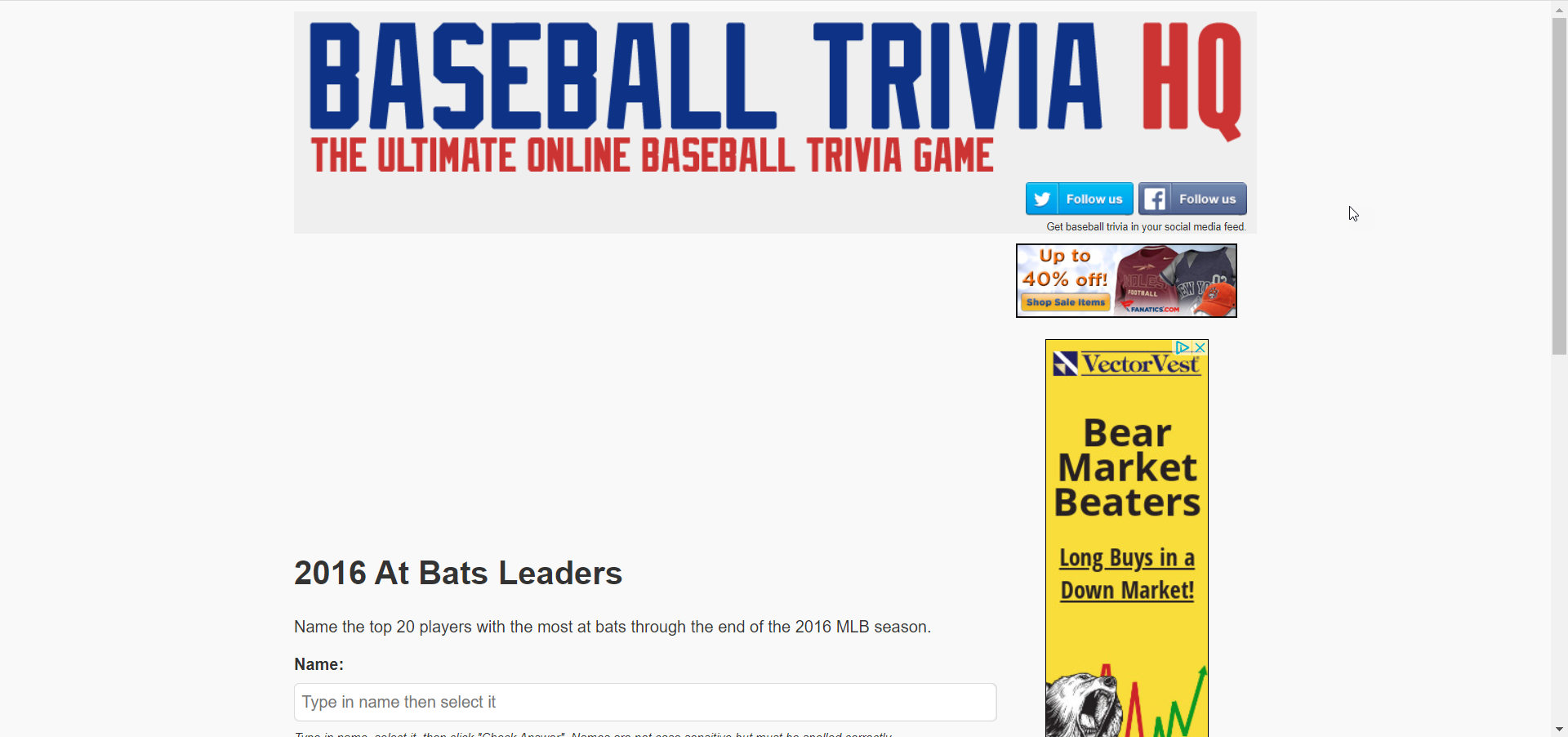
For this segment, we'll work with the At Bat leaders (AB) for 2016.
Source: Baseball Trivia HQ
What I like about this type of trivia quiz is that it shows you the AB numbers for the top 20 leaders for 2016 and you have to guess the player for each spot.
The task is to create code with dplyr commands to match the numbers in the table. Then, you can fill in each of the names as they appear from the results of the code.
The exercise is valuable not just for getting the right answers for the quiz but also for validating that the code you create produces the correct numbers.
To reduce the complexity of this task, let's create an object that is a subset for 2016 of the batting table. In dplyr it's as easy as the following:
batting2016 <- Batting %>% filter(yearID == 2016)
Next, we'll need to capture the players who had the highest at bats (AB) for 2016. The following may seem like it would do the trick:
batting2016 %>% arrange(desc(AB))
At first glance, it seems like we nailed it and got the correct numbers. However, if you look close, you'll see that the 623 in the Baseball Trivia HQ table is missing in our output from the code.
The player who had 623 at bats in 2016 is Matt Kemp. When looking up the stats for Matt Kemp in 2016:

Matt Kemp played on two teams that year, the San Diego Padres (SDN) and the Atlanta Braves (ATL). The question doesn't ask for the at bats broken out by team for 2016. It asks for at bats for 2016. That means we need to add up players' total stats for the year.
Most players only played for one team which is why this situation didn't happen to those other players. To handle this situation for any player going forward, we'll group by the player and summarize (using sum) the total at bats. Hence:
batting2016 %>%
group_by(name) %>%
summarize(sumab = sum(AB)) %>%
arrange(desc(sumab))
This command is described as follows:
Use the prefiltered 2016 records (from above) and pipe that into the group_by statement. Use name as the field to group. Pipe the result of this into the summarize statement. The sum() function is used to get a sum of at bats for the player for 2016. Finally, pipe the result of that to the sort (arrange) function, and sort it in descending order.
Now, let's take a look at the results:
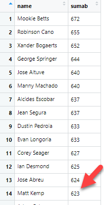
This matches exactly with the chart in Baseball Trivia HQ. Go ahead and check. You'll see that it matches.
You may notice that the results drop several fields in the batting2016 table. This is what happens with aggregations. Since we only asked to summarize at bats that are grouped by name, the output only includes the name and the summarized at bats.
Anyone Ever Hear of Al Smith in Baseball?
This is a good place to explain why grouping by name only is dangerous.
If you were alive to watch baseball in 1926, you probably heard of a player named Al Smith. He played one game his entire career. For reference, his playerID is smithal02.
There is a player with playerID smithal01. His name is Aleck Smith. He wouldn't affect this discussion as he wouldn't appear as part of grouping the name Al Smith.
If you watched baseball in the 1930s, you also may have caught a player named Al Smith. This Al Smith started in 1934 and played until 1945. His playerID is smithal03.
Finally, in the 1950s, another Al Smith played the game. He played from 1953 to 1964, and his playerID is smithal04.
Now that we have the name field added to the tables, it seems logical to group by the name field. If we grouped by playerID, the name field would be lost during the aggregation. We would then have to create some kind of lookup between playerID and People table, which is cumbersome.
Why not just use playerIDs? Although some playerIDs are obvious, like ruthbabe01, many are not. Having the player name as part of the results is a huge plus.
To see for yourself why this is a problem, try the following queries:
Batting %>% group_by(name) %>% filter(name == 'Al Smith') %>% summarize(sum(G))
Batting %>% group_by(playerID) %>% filter(name == 'Al Smith') %>% summarize(sum(G))
The first query (group by name) lumps all three Al Smiths together as if they were one person. The output should be three rows, one for each of the three Al Smiths. It's a valid query though, even if the data is nonsensical.
The second query (group by playerID) gives the correct results. Three summaries, one for each player. Totally makes sense.
What's even worse about this situation is that your queries may work when grouping by name, depending on what you enter. In other words, grouping by name will produce the same results as grouping by playerID in many cases. Then, you'll run a query that produces the wrong results. Since it is a valid query though, it may go undetected.
To fix this problem and still include the player name, simply group by both, starting with the playerID first, like so:
Batting %>% group_by(playerID, name) %>% filter(name == 'Al Smith') %>% summarize(sum(G))
I urge you to take the time to understand the difference and why it matters.
You could accomplish the same with this:
c(10, 20, 15) %>% mean()
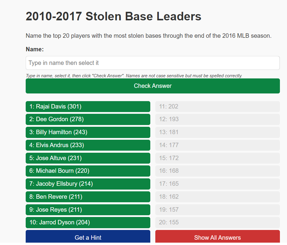
2010-2017 Stolen Base Leaders
To find out the leaders for a block of years, it isn't much different than the previous item. But this time, we won't create a subset object for the years, like we did for batting2016, although you are welcome to do that if it's easier for you conceptually.
As the queries get more complex, you'll want to think about what you're trying to accomplish. For this, we'll need an aggregation of years from 2010-2017. We're not dealing with any particular team, but we'll still need to group by players (name) to account for players who played for multiple teams in one year.
We'll use the Batting table instead of batting2016 table. This is because we need more of years data. See if you can find which field we need in the Batting table. You can find a list of columns using the str() command:
str(Batting)
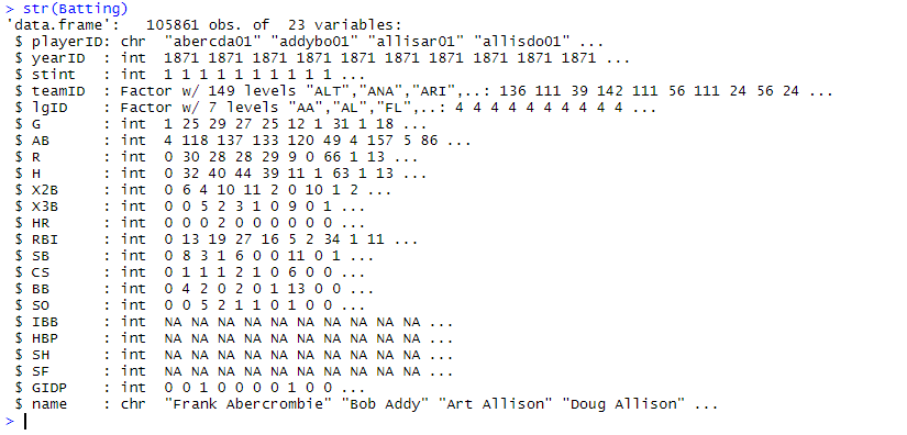
As you can see, the one that would make the most sense would be the SB field. If you are unsure, most database will make their help available describing the fields:
?Batting
Sure enough, SB is the stolen bases field.
Here is a stab at the code:
Batting %>%
filter(yearID >= 2010 & yearID <= 2017) %>%
group_by(playerID, name) %>%
summarize(sumsb = sum(SB)) %>%
arrange(desc(sumsb))
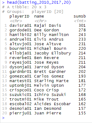
You'll notice in the results window I wrapped the above query in a head() command. This is useful to print out only the top 20 results. The head() command will display six results by default unless you append the number of rows you want to display. Hence, the ",20" at the end of the statement.
You can check your results against the Baseball Trivia HQ page:
Feel free to enter all the names returned from the query and see that they match.
Conclusion
I thought about adding some more examples, but this tutorial is getting rather bloated and adding more may muddy the waters, if you will. Besides, you'll want to keep the queries simple in the beginning.
Do you need to use baseball trivia for this tutorial? Of course not! If you find other sources of information or are just playing around with different queries, it is not required.
What I like about using trivia sites is you can tie out the numbers. This trivia website gives you the numbers that should be the results. You have only to keep trying some queries until you answers match.
I honestly believe DPLYR is simple enough a library for you to use (and powerful). In most cases, you'll need the filter, group_by, summarize, and arrange. Just keep using these until they become second nature. The format doesn't change.
Just use information that is specific to the question you want answered. Change the year, or filter by a specific player (Babe Ruth, anyone?). The summarize is likely to contain the sum() function. On occasion, you may need to use mean() instead.
Most people will search for queries with the best players in a category, like shown in this article. The arrange(desc()) construct helps with this. If you wanted to discover worst, just leave out the desc() in the arrange command.
The last point to make is that you'll need to grasp the pipe operator. But that's easy, too! Take the results from one query and 'pipe' it using (%>%) into another query. The pipe replaces the first parameter in the next query.
If you have any questions whatsover about this tutorial, feel free to provide them in the comments below.

